clc,clear;
% 对x轴部分
x(1) = 0;
x(9) = 1;
for i = 7:-1:1
x(9-i) = 1/(2^i);
end
% 对y轴部分
y = 0:1/8:1;
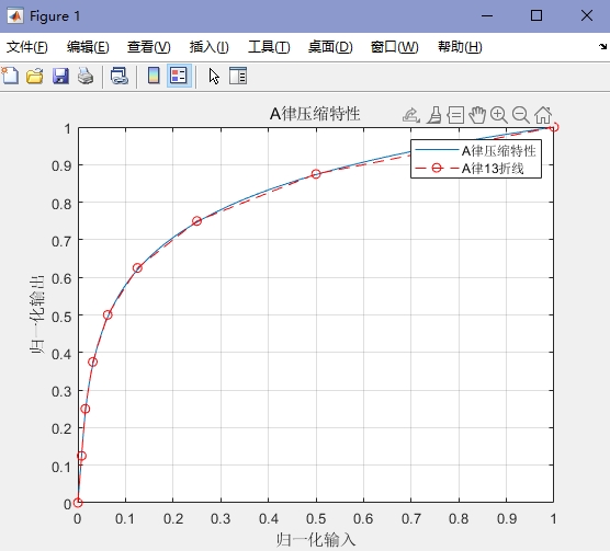
% A律特性
A = 87.6;
dt = 1/1000;
xx = 0:dt:1;
for i = 1:length(xx)
if xx(i) <= 1/A;
yy(i) = A*xx(i)/(1+log(A));
else
yy(i) = (1+log(A*xx(i)))/(1+log(A));
end
end
% 画图
plot(xx, yy);hold on
plot(x, y, 'ro--');hold on
xlabel('归一化输入');ylabel('归一化输出');title('A律压缩特性');grid
legend('A律压缩特性','A律13折线')
实验效果
两路径无线信道模型仿真
实验代码
clc,clear;
% 参数设置
p = [0.99 0.9];
N = 1000;
d = 5;             %延时样本数
for i = 1:length(p)
    A = [1 -2*p(i) p(i)^2];        %滤波器参数
    B = (1-p(i))^2;
    white_noise_seq1 = randn(1,N);
    white_noise_seq2 = randn(1,N);
    R1(i, :) = filter(B, A, white_noise_seq1);
    R2(i, :) = filter(B, A, white_noise_seq2);
    h(i, :) = R1(i,d+1:N)+R2(i,1:N-d);
end
subplot(2, 1, 1);
plot(1:N,R1(1, :),'-',1:N,R2(1, :),'--',1:N-d,h(1, :),':');
legend('径1', '径2', '合成信道')
xlabel('n');ylabel('幅度');title('p=0.99')
subplot(2, 1, 2);
plot(1:N,R1(2, :),'-',1:N,R2(2, :),'--',1:N-d,h(2, :),':');
legend('径1', '径2', '合成信道')
xlabel('n');ylabel('幅度');title('p=0.9')
实验效果
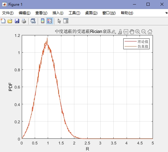
产生受遮蔽的Rician衰落分布的信道系数
实验代码
clc,clear;
% 产生对数分布均值的复高斯随机变量
N = 10^5;     % 样值点数
sigma_a = 0.252;    % 散射信号分量方差
x = sqrt(sigma_a/2)*randn(2, N);
sigma_z = 0.161^2;   % 直射信号分量对数的方差
u_z = -0.115;        % 直射信号分量对数的均值
zz = sqrt(sigma_z)*randn(1, N);
z = exp(zz +u_z);
xx = z + x(1, :) + sqrt(-1)*x(2, :);
k = 0:0.01:5;
pdf_sim = c_pdf(k, abs(xx));
% 理论值
kk = 0:0.01:5;
dz = 0.001;
zk = dz:dz:10;
for i = 1:length(kk)
    xa = 2*kk(i)/(sqrt(2*pi*sigma_z)*sigma_a);
    xb = exp(-(kk(i)^2+zk.^2)/sigma_a-(log(zk)-u_z).^2/(2*sigma_z));
    xc = besseli(0, 2*kk(i)*zk/sigma_a)*dz./zk;
    xd = sum(xb.*xc);
    pdf_lilun(i) = xa*xd;
end
% 画图
plot(kk, pdf_lilun, 'r');hold on
plot(k, pdf_sim, '-');grid
xlabel('R');ylabel('PDF');legend('理论值', '仿真值');
title('中度遮蔽的受遮蔽Rician衰落分布')
clc,clear;
echo on
clear;
t0=.2; % signal duration
ts=0.001; % sampling interval
fc=250; % carrier frequency
snr=20; % SNR in dB (logarithmic)
fs=1/ts; % sampling frequency
df=0.3; % required freq. resolution
t=[-t0/2:ts:t0/2]; % time vector
kf=100; % deviation constant
df=0.25; % required frequency resolution
m=sinc(100*t); % 消息信号
int_m(1)=0;
for i=1:length(t)-1 % integral of m
int_m(i+1)=int_m(i)+m(i)*ts;
echo off ;
end
echo on ;
[M,m,df1]=fftseq(m,ts,df); % 傅里叶变换
M=M/fs; % scaling
f=[0:df1:df1*(length(m)-1)]-fs/2; % frequency vector
u=cos(2*pi*fc*t+2*pi*kf*int_m); % 已调信号
[U,u,df1]=fftseq(u,ts,df); % Fourier transform
U=U/fs; % scaling
[v,phase]=env_phas(u,ts,250); % 解调,找到u的相位
phi=unwrap(phase); % 还原原始的相位
dem=(1/(2*pi*kf))*(diff(phi)/ts); % 解调输出, differentiate and scale phase
% pause % Press any key to see a plot of the message and the modulated signal.
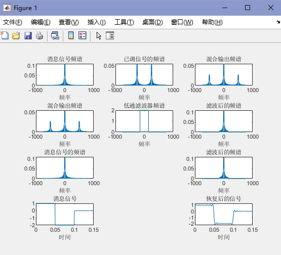
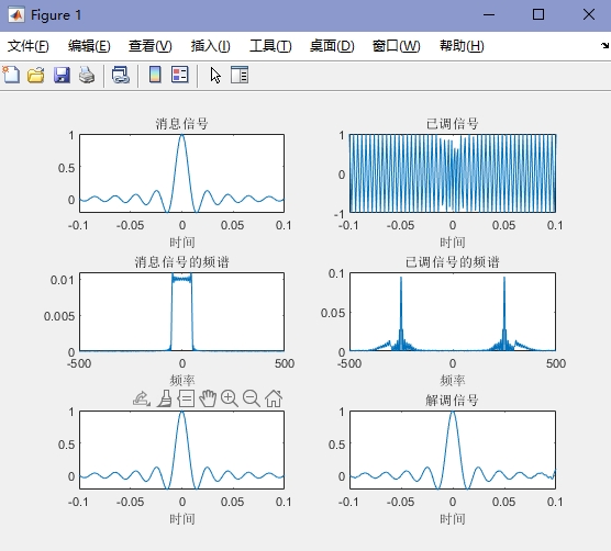
subplot(3,2,1)
plot(t,m(1:length(t)))
xlabel('时间')
title('消息信号')
subplot(3,2,2)
plot(t,u(1:length(t)))
xlabel('时间')
title('已调信号')
% pause % Press any key to see plots of the magnitude of the message and the
% modulated signal in the frequency domain.
subplot(3,2,3)
plot(f,abs(fftshift(M)))
xlabel('频率')
title('消息信号的频谱')
subplot(3,2,4)
plot(f,abs(fftshift(U)))
title('已调信号的频谱')
xlabel('频率')
% pause % Press any key to see plots of the message and the demodulator output with no
% noise.
subplot(3,2,5)
plot(t,m(1:length(t)))
xlabel('时间')
title('消息信号')
subplot(3,2,6)
plot(t,dem(1:length(t)))
xlabel('时间')
title('解调信号')
实验效果
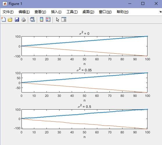
解说题7.9 QAM信号的解调
实验代码
clc,clear;
M = 8;
Es = 1;
T = 1;
Ts = 100/T;
fc = 30/T;
t = 0:T/100:T;
l_t = length(t);
A_mc = 1/sqrt(Es);                      % 信号幅度
A_ms = -1/sqrt(Es);                     % 信号幅度
g_T = sqrt(2/T)*ones(1,l_t);
phi = 2*pi*rand;
si_1 = g_T.*cos(2*pi*fc*t + phi);
si_2 = g_T.*sin(2*pi*fc*t + phi);
var = [ 0 0.05 0.5];                    % 噪声方差矢量
for k = 1 : length(var)
    % 噪声成分的产生:
    n_c = sqrt(var(k))*randn(1,l_t);
    n_s = sqrt(var(k))*randn(1,l_t);
    noise = n_c.*cos(2*pi*fc+t) - n_s.*sin(2*pi*fc+t);
    % 接收到的信号
    r = A_mc*g_T.*cos(2*pi*fc*t+phi) + A_ms*g_T.*sin(2*pi*fc*t+phi) + noise;
    % 相关器输出:
    y_c = zeros(1,l_t);
    y_s = zeros(1,l_t);
    for i = 1:l_t
        y_c(i) = sum(r(1:i).*si_1(1:i));
        y_s(i) = sum(r(1:i).*si_2(1:i));
    end
    % 绘制结果:
    subplot(3,1,k)
    plot([0 1:length(y_c)-1],y_c,'.-')
    hold
    plot([0 1:length(y_s)-1],y_s)
    title(['\sigma^2 = ',num2str(var(k))])
    xlabel('n')
    axis auto
end
实验效果
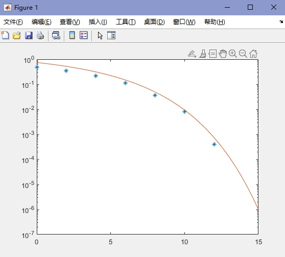
解说题7.10 QAM信号的仿真
实验代码
clc,clear;echo on
SNRindB1=0:2:15;
SNRindB2=0:0.1:15;
M=16;
k=log2(M);
for i=1:length(SNRindB1)
    smld_err_prb(i)=cm_sm41(SNRindB1(i));	% 模拟错误率
    echo off;
end
echo on ;
for i=1:length(SNRindB2)
    SNR=exp(SNRindB2(i)*log(10)/10);    	% 信噪比
    % 理论符号错误率
    theo_err_prb(i)=4*Qfunct(sqrt(3*k*SNR/(M-1)));
    echo off ;
end
echo on ;
% 绘图
semilogy(SNRindB1,smld_err_prb,'*');
hold
semilogy(SNRindB2,theo_err_prb);
实验效果
解说题8.2 OFDM信号的产生
实验代码
clc,clear;echo on
K=10;N=2*K;T=100;
a=rand(1,36);
a=sign(a-0.5);
b=reshape(a,9,4);
% 生成16QAM点
XXX=2*b(:,1)+b(:,2)+1i*(2*b(:,3)+b(:,4));
XX=XXX';
X=[0 XX 0 conj(XX(9:-1:1))];
xt=zeros(1,101);
for t=0:100
    for k=0:N-1
        xt(1,t+1)=xt(1,t+1)+1/sqrt(N)*X(k+1)*exp(1i*2*pi*k*t/T);
        echo off
    end
end
echo on
xn=zeros(1,N);
for n=0:N-1
    for k=0:N-1
        xn(n+1)=xn(n+1)+1/sqrt(N)*X(k+1)*exp(1i*2*pi*n*k/N);
        echo off
    end
end
echo on
plot(0:100,abs(xt))
% 检查xn与x(t)样本之间的差异
for n=0:N-1
    d(n+1)=xt(T/N*n+1)-xn(1+n);
    echo off
end
echo on
e=norm(d);
Y=zeros(1,10);
for k=1:9
    for n=0:N-1
        Y(1,k+1)=Y(1,k+1)+1/sqrt(N)*xn(n+1)*exp(-1i*2*pi*k*n/N);
        echo off
    end
end
echo on
dd=Y(1:10)-X(1:10);
ee=norm(dd);
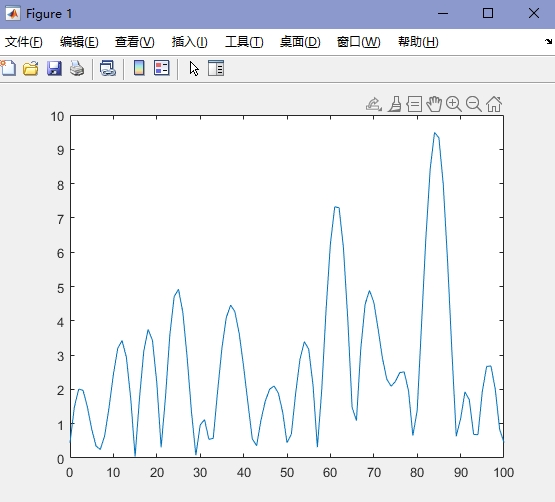
实验效果
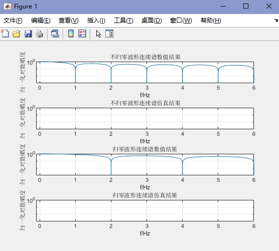
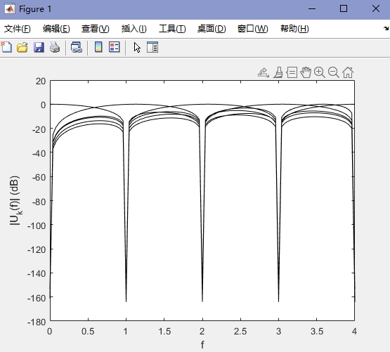
解说题8.5 OFDM信号的频谱
实验代码
clc,clear;
T = 1;
k = 0 : 5;
f_k = k/T;
f = 0 : 0.01*4/T : 4/T;
U_k_abs = zeros(length(k),length(f));
for i = 1 : length(k)
    U_k_abs(i,:) = abs(sqrt(T/2)*(sinc((f-f_k(i))*T) + sinc((f+f_k(i))*T)));
    U_k_norm(i,:) = U_k_abs(i,:)/max(U_k_abs(i,:));
end
U_k_dB = 10*log10(U_k_norm);
plot(f,U_k_dB(1,:),'black',f,U_k_dB(2,:),'black',f,U_k_dB(3,:),'black',...
    f,U_k_dB(4,:),'black',f,U_k_dB(5,:),'black',f,U_k_dB(6,:),'black')
axis([min(f) max(f) -180 20])
xlabel('f')
ylabel('|U_k(f)| (dB)')
实验效果
全部子函数
实验代码
%% 高斯分布函数
function[y] = normal_pdf(x, m, sigma)
% 产生均值为m,方差为sigma的高斯分布函数
% x取值区间为[a b]
y = exp(-(x-m).^2/(2*sigma))/sqrt(2*pi*sigma);
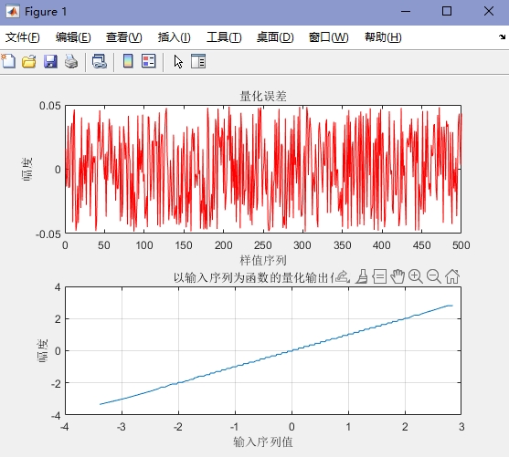
%% 均与量化与自然编码子程序,x -- 模拟信源, n -- 量化级数
function[x_q, code, delat] = unipcm(x, n)
M = log2(n);
x_width = max(x) - min(x); % 量化范围的大小
delat = x_width/n; % 量化间隔
xx = min(x):delat:max(x); % 量化分层电平值
q = min(x) + delat/2:delat:max(x); % 量化电平值
for i = 1:length(x)
if x(i) <= xx(2) % 小于等于第2个量化分层的均属于第1量化级
x_q(i) = q(1);
index(i) = 1;
end
k = 2;
while k < n+1
if(x(i) > xx(k)) & (x(i)<=xx(k+1)) % xx(k) < x(i) <= xx(k+1),位于分层电平
index(i) = k;
x_q(i) = q(k);
k = n+1;
end
k = k+1;
end
code(i*M:-1:(i-1)*M+1) = de2bi(index(i)-1, M); % 二进制编码
end
function pdf = c_pdf(k, data)
[counts, binCenters] = hist(data, k);
pdf = counts / (sum(counts) * (binCenters(2) - binCenters(1)));
end
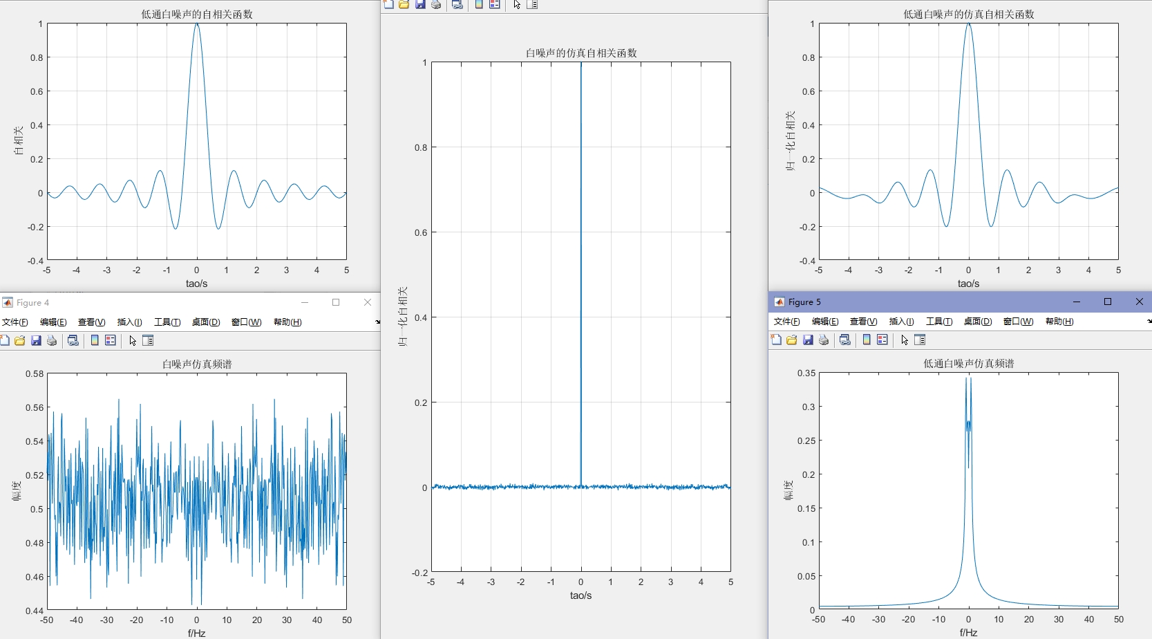
function Rx = Rx_est(x, M)
% 计算自相关函数
N = length(x);
Rx = zeros(1, M+1);
for m = 0:M
Rx(m+1) = sum(x(1:N-m) .* x(m+1:N)) / N;
end
end
function xl=loweq(x,ts,f0)
% xl=loweq(x,ts,f0)
%LOWEQ returns the lowpass equivalent of the signal x
% f0 is the center frequency.
% ts is the sampling interval.
%
t=[0:ts:ts*(length(x)-1)];
z=hilbert(x);
xl=z.*exp(-j*2*pi*f0*t);
function [M,m,df]=fftseq(m,ts,df)
% [M,m,df]=fftseq(m,ts,df)
% [M,m,df]=fftseq(m,ts)
%FFTSEQ generates M, the FFT of the sequence m.
% The sequence is zero padded to meet the required frequency resolution df.
% ts is the sampling interval. The output df is the final frequency resolution.
% Output m is the zero padded version of input m. M is the FFT.
fs=1/ts;
if nargin == 2
n1=0;
else
n1=fs/df;
end
n2=length(m);
n=2^(max(nextpow2(n1),nextpow2(n2)));
M=fft(m,n);
m=[m,zeros(1,n-n2)];
df=fs/n;
function [v,phi]=env_phas(x,ts,f0)
% [v,phi]=env_phas(x,ts,f0)
% v=env_phas(x,ts,f0)
%ENV_PHAS Returns the envelope and the phase of the bandpass signal x.
% f0 is the center frequency.
% ts is the sampling interval.
%
if nargout == 2
z=loweq(x,ts,f0);
phi=angle(z);
end
v=abs(hilbert(x));